LOFT: Learned Open Flow-based Tracking

Qingyuan Li	Alexandru Luchianov
Final project for MIT 6.7960

Example frame from our algorithm. Outputs from top left, clockwise: RGB image with annotated dynamic objects, depth image, raw model output mask, post-processed model output mask.

Preface

One of the previous projects of Qingyuan Li involved dynamic object tracking by using the flow residual information, however the result was lacking. This section aims to provide context as to what the previous approach did, why it failed and why deep learning is the solution.

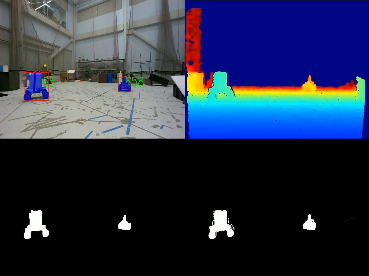
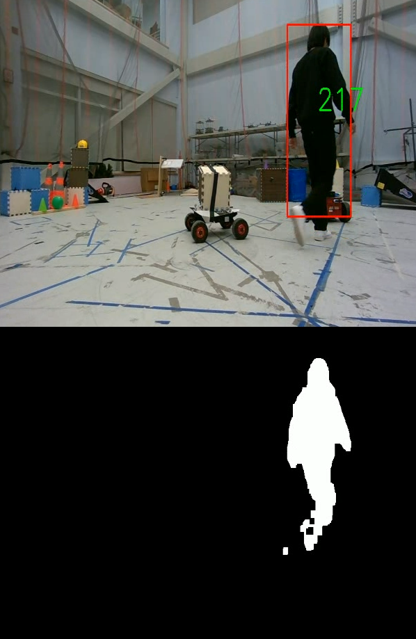
In very succinct terms, the core pipeline of the previous project could be described as such:

1. Gather data for the dynamic object tracking experiment.
2. Extract the optical flow from the image using a known model(RAFT)
3. Process the optical flow and the original frame to obtain the objects

The idea seems simple in practice, so simple, in fact, that this project could also be described by a similar list of steps. However, "processing the optical flow" hides a lot of abstraction underneath. In the previous project, this processing meant tagging every pixel that is moving faster than a certain velocity as a "dynamic object" and then merely post-processing the binary mask with OpenCV morphological operations in order to remove the noise. This game of post-processing was akin to Whac-a-mole, opening an image would remove small points of noise, closing would remove small holes, but the noise would still be noticeable. (See Video 1 for an example.) The winning strategy of this game was, obviously, not to play at all. For this project, we decided that a model is much better suited at learning what set of transformations would be best.

Video 1. Example output sequence from the evaluation dataset with the non-learned algorithm

Unfortunately, replacing the manual transformation of data by a learning model subtly (and signficantly) changes the other steps of the pipeline too. The most significant change was that of what ground truth is necessary. In the previous iteration of the project our evaluation metric was merely whether the detected location of the object was close enough to where we know the object to be. However, our segmentation model requires the whole segmentation of the object as a ground truth.

We could not collect this ground truth as we were only able to collect data about the approximate pose of the objects. Note that if we had the shape of the objects, we would have been able to generate the ground truth by simply projecting them. Our solution is to generate the ground truth using the Segment Anything model ([2]) and then train our smaller model on that. Note that training on this synthetic data makes our model inherently less accurate than SAM, however our model is much lighter.

Motivation

Unmanned Aerial Vehicles and Unmaned ground vehicles have numerous applications in fields such as delivery, photography, monitoring and many others. However, being unmanned leaves them dependent on signal coverage and a stable connection in order to be teleoperated by an operator. In order to overcome this limitation, much effort has been directed towards the issue of autonomous control.

Unfortunately, autonomous control has its own set of limitations. Where a human would be able to operate with only limited signal, an autonomous device often requires significantly more sensors. For example, a Waymo car employs a total of 29 cameras and possesses Lidar capabilities. This extensive payload is the reason why adoption is limited even for low-risk applications.

We aim to provide a lightweight solution for performing real-time dynamic obstacle recognition.

Related works

Segmentation is an extremely broad field that has spawned many diverse tasks. In order to tackle the ever-expanding nature of the field, significant time and effort has been invested in creating capable models that can adapt to many of these existing tasks. One of the most prominent and succesful examples of such a project is the Segment Anything ([2]) model. Naturally, the model's core strength, its generality, is also its core weakness as it cannot properly take advantage of highly specific advantages. To put this into our context of Video Object Segmentation, SAM(Segment Anything Model) cannot take advantage of the information that is inherent in the video format and must segment each frame independently.

A more recent work that tries to bridge this gap is [1]. Instead of ignoring the information from the video feed itself, it tries to feed the optical flow either as an input (by converting it to an RGB image) or to create prompts for the original image. While this approach does not discard the useful data from the video, it achieves its purpose in a roundabout way that avoid training a new model and thus not really specializing. Another significant disadvantage acknowledged by the authors of the paper: SAM is computationally heavy, thus the resulting model is also extremely slow. In contrast, our model is trained and specialized, thus is can be much lighter and efficient.

[4] and [3] further generalize the SAM model, thus allowing it to to process videos. Note that this advancement obsoletes the papers that merely provide a wrapper around SAM in order to provide it with additional video capabilities. Unfortunately, SAM is still a massive model that is extremely computationally expensive and thus impractical for our purposes. However, we do note that it is still a key component of our pipeline that allows us to cheaply and reliably generate ground truths for our collected training data.

[10] further augments SAM by providing semantic context from DINO([11]) features. While this approach achieves really high accuracy, that is achieved at the cost of speed. We considered using DINO features with our model, however we ultimately decided against it due to DINO feature vectors being really long and not compatible with our idea of creating a lightweight model.

An example of a lightweight model that makes use of optical flow is RST-MODNet ([9]). This model uses a LSTM-based network in order to leverage the temporal information to a stronger degree. The disadvantage of this approach is that the recurrent nature of the network makes it really computationally expensive to train. Another significant difference is that they use the raw optical flow, rather than the residual flow which accounts for the movement of the observer.

We note that most of these works build upon image segmentation towards video segmentation and that advacements in the former also tend to provide advancements in the latter. However, this relationship is not unidirectional and sometimes advancements in video segmentation can provide advancements in image. [5] provides a framework for generating synthetic flows from depth data. This enables models that are reliant on optical flow cues to provide similar results when tested on static images. Specifically, this implies that our work can be further generalized to static images.

Model inputs

As one of the main ingredients, it is natural that we dedicate some of our attention to the problem of optical flow. Due to it being a relatively common problem there exist pretty performant solutions such as RAFT ([6]). We additionally remark that not only is RAFT one of the solutions, it is the primary solution to the problem of optical flow, being at the base of most of the related works. Even though optical flow can be summarized roughly as "how did a pixel move between frames" and then used as blackbox, we consider that some context about this "black box" could help us make an informed decision about the rest of our architecture.

Formally, optical flow solves the below optimization problem: \[ E = \min_{\mu} \left[ (\nabla^T \mathbf{I}_1\mu - (\mathbf{I}_2-\mathbf{I}_1)^2+\alpha(|\nabla \mu_x|^2+|\nabla \mu_y|^2)) \right] \]

There are two core assumptions that motivate the above formulation:

1. Color constancy: Pixels won't spontaneously change colors.
2. Velocity averaging: Nearby pixels move together.

Obviously, these assumptions are not universal truths and one can construct scenarios in which they do no hold ranging from the most contrived (we are trying to follow a chameleon or every pixel has a mind of its own and running independently) to quite mundane things (lighting conditions change or it is raining). In our case, we performed our data collection in an indoor environment where such anomalies can be controlled and minimized.

A pitfall of the optimization problem formulation is that often we don't have only two adjacent frames, but rather an entire video. Solving an optimization problem for each two adjacent frames would be extremely computationally expensive. RAFT circumvents expensive computation by extracting per-pixel features and building multi-scale 4D correlation volumes. Aside from the efficiency gains, this representation confers it some additional robustness against lighting changes and blur.

For the sake brevity, we will only provide a description of each of the model inputs. (For an actual derivation of them, please refer to the appendix):

• RAFT Flows 2D: Flow of a pixel from the previous frame to the current frame as computed by RAFT
• Geometric Flow 2D: Flow of a pixel if we assume that the background is static and we account only for the camera movement.
• Residual 2D: The difference between the RAFT flow and the geometric flow. This represents the actual movement in 2-dimensional space induced by the object, not by the camera.
• RAFT Flows 3D: Flow of a pixel from the previous frame to the current frame as computed by RAFT plus the depth information.
• Geometric Flows 3D: Flow of a pixel in 3-dimensional space if we assume that the background is static and we account only for the camera movement.
• Residual Flow 3D: The difference between the RAFT flow and the geometric flow. This represents the actual movement in 3-dimensional space induced by the object, not by the camera.
• Depth Data: Depth information for each pixel. Note that this is capped at 6m meters due to the limitations of our sensors.
• RGB Data: The raw RGB image.

These inputs will be later fed into the U-Net in the form of an image with enough channels for all of the above.

U-Net

Image segmentation is a notoriously hard problem to annotate data for. Rather than trying to annotate an ever-increasing amount of data, some projects have opted for trying to make more efficient use of the existing annotated data. This has led to the creation of the U-Net ([7]). Aside from their efficiency in terms of training data, these models are small, fast and reliable. This makes them a natural choice of a base on which to build our custom model.

A succinct description of the U-net architecture is that it consists of a contracting path and an expansive path. The contractive path reduces the resolution of the image by downsampling while adding more channels in order to propagate context. The expansive path does the exact opposite: it upsamples while reducing the number of channels. This leads the network to have a "U" structure, thus providing it with its name. The details of the paths are more easily apparent in the visual reminder of the U-Net architecture that we also provide below in the form of Figure 1:

Figure 1: The U-Net Architecture.

The main distinction between the traditional architecture and ours is that instead of using a traditional RGB image, we instead add additional channels that provide additional context. This additional context is mostly either depth information or optical flow information. Note that optical flow itself also can be presented in many ways such as either 3-dimensional, 2-dimensional, RAFT flow or geometric flow.

We use the Dice coefficient in order to evaluate the outputs of the U-Net and train it. We note that this metric only measures the quality of the segmentation which is merely an intermediate product. The overall metric that we use for dynamic object detection is different. We remind that the dice formula is $$DSC = \frac{2|X \cap Y|}{|X| + |Y|}$$ If our collected data was free of noise, then X would be the set of segmented pixels in the ground truth and Y would be set of segmented pixels in the output of our model. However, due to imperfect collection of data some of our depth pixels were nan. In order to account for the errors of our equipment, we only included the unaffected pixels in this metric.

The specific U-Net implementation on which we based our work can be found here at [8].

Dataset colection

We collected all of the training and evaluation data at the Highbay of the Aerospace Controls Laboratory at MIT. This controlled environmnet provided us with stable lightning and weather conditions in order for the optical flow to be easy to detect accurately, and contains a ground truth motion capture system for evaluation. We remind that our aim is to measure the efficacy of the techniques applied for the processing of optical flow and image data, not to optimize optical flow detection itself.

In terms of hardware, we used a RealSense D455 depth camera on a Clearpath Husky with an Ouster lidar and MicroStrain IMU running lidar-inertial odometry. The moving objects are teleoperated hexcopter and another ground robot.

The ground truth pose data was collected using a Vicon motion capture system and recorded in a ROS2(Robot Operating System) bag. The Husky recorded a ROS1 bag with depth camera and pose data. We use our own ROS bag processing software for dataloading. Note that the ground truth collected above only provided pose information. Ground truth pose information combined with a rought estimate of the shapes of the robots allowed us to compute approximate bounding boxes. This allowed us to use SAM([2]) with bounding box-guided prompts to generate ground truth for the image segmentation.

Metrics

We used the standard precision and recall metrics in order to quantify the performance of our model. Note that since ground truth data and visual data are collected by different machines, there might exist discrepancies gaps in the collected timestamps. In order to account for this, we only compute the metrics for frames for which there exists a close enough ground truth. Let the model return a list of detected dynamic objects and their poses.

We consider an object to be relevant only if we could feasibly detect it and the detected position is close to the true location (within one meter). By feasibly detect, we mean that we only consider objects that are both moving with high enough velocity (at least 0.1 m/s) and whose centroid lies within the boundary of the current image frame. Based on this definition of relevant we provide the following metrics:

• Precision: The ratio of returned objects that actually are relevant (actually exist and could be detected)
• Recall: The ratio of relevant objects(that actually exist and could be detected) that were actually returned

All evaluations were run with the RAFT Sintel model. Opening and closing with a 9x9 kernel were used as morphological operations for post-processing all binary masks to reduce point noise. Objects with a maximum standard deviation below 0.05m or above 1.0m are ignored. Objects beyond the depth range are also ignored.

Evaluation

Model	RAFT Flows 2D	Geometric Flow 2D	Residual 2D	RAFT Flows 3D	Geometric Flows 3D	Residual Flow 3D	Depth (Cur)	RGB (Cur)	Depth (Prev)	RGB (Prev)
Non-learned	✗	✗	✗	✗	✗	✗	✗	✗	✗	✗
1xRGBD Only	✗	✗	✗	✗	✗	✗	✓	✓	✗	✗
1xRGBD + 2d Residuals	✗	✗	✓	✗	✗	✗	✓	✓	✗	✗
1xRGBD + 3d Residuals	✗	✗	✗	✗	✗	✓	✓	✓	✗	✗
2xRGBD Only	✗	✗	✗	✗	✗	✗	✓	✓	✓	✓
2xRGBD + 2d Residuals	✗	✗	✓	✗	✗	✗	✓	✓	✓	✓
2xRGBD + 3d Residuals	✗	✗	✗	✗	✗	✓	✓	✓	✓	✓
2xRGBD Full	✓	✓	✓	✓	✓	✓	✓	✓	✓	✓

Model	Dice coefficient	Recall	Precision
Non-learned	0.475	0.713	0.320
1xRGBD Only	0.440	0.973	0.510
1xRGBD + 2D Residuals	0.499	0.934	0.499
1xRGBD + 3D Residuals	0.478	0.886	0.424
2xRGBD Only	0.491	0.908	0.523
2xRGBD + 2D Residuals	0.474	0.936	0.468
2xRGBD + 3D Residuals	0.464	0.940	0.462
2xRGBD Full	0.528	0.904	0.538

Video 2. Example output sequence from the evaluation dataset (2xRGBD Full)

The full evaluation video for 2xRGBD Full can be found here.

Conclusion

We observed significantly better results with the model-based approaches when compared to the original non-learned algorithm in both precision and recall, achieving our objective of real-time dynamic object detection with high accuracy.

We note that the recall of the models was significantly higher than their precision. Based on examination of the videos, we reached the conclusion that this is due to noisy frames with many false positives in which the RAFT and geometric flow significantly diverge, most likely due to noisy odometry or depth. This leads the whole frame to become noisy, thus possibly detecting many more objects in the image. In our training and evaluation data there are at most 2 objects, thus there is only so many false negatives that one can incur per frame, and our models tend to be aggressive in their detections.

Interestingly, and perhaps somewhat expectedly, the model that only uses RGBD data without any flow information already outperforms the non-learned method by a large margin. Therefore, much of this improvement can probably be attributed to the model learning how to detect robots (moving or not) from the RGB and depth data alone. Still, the model that used all of the inputs outperformed all other methods in Dice coefficient and precision, suggesting that the optical flow residuals do provide useful information for the task of dynamic object detection. These specific improved metrics suggest that the model is better able to distinguish between moving and static robots, thus slightly reducing false positives (though not significantly, because of the high noise ratio), which reflects the value of the optical flow information. To better understand this behavior, we would need to collect and train on data in which the robots do not move a majority of the time.

As seen in Figure 2, the model also generalizes to humans, despite never having seen any human data during training, suggesting highly promising generalization capabilities.

Figure 2: a moving human being detected

We believe that the performance of our models could be further improved by providing them with additional training data and more training time, especially due to the high false positive rate. Given how hard it is to generate meaningful training data, data augmentation methods should be explored in order to allow for creating larger datasets from pre-existing data. To leverage the additional data, a more complex model, possibly using attention mechanisms, could be explored as well. However, model complexity would likely come at the cost of inference speed.

Another area of improvement could be to improve temporal consistency. Currently, each sequence of two frames is treated independently, however, in practice, temporal consistency could provide significant improvements. Methods such as LSTMs or 3D convolutions could be explored for this purpose. Again, these methods would likely slow the method down significantly.

In conclusion, we believe that our method provides a lightweight and efficient solution for dynamic object detection. Future work could explore more complex models and temporal consistency in order to further improve performance, but over 90% recall and over 50% precision is a promising result for a model trained from scratch with limited data.

Codebase

See [dynamic-object-detection on Github] for our implementation. Instructions for downloading our data and running the algorithm and evaluations are in the README. Note that this repository only contains the code responsible for the dynamic object detection side of things. Our fork of the U-Net repository is linked as a submodule and contains more training and evaluation information.

Acknowledgements

We would like to thank Professor Jonathan How for his guidance throughout this project and for generously providing access to the resources that we utilized. Special thanks as well to Lucas Jia for assisting us with physical experiments, data collection and providing us with hardware powerful enough to train our model.

Appendix

This analysis of the difference between the RAFT optical flow and geometric optical flow is reproduced from the previous project.

We obtain our flow residuals by computing the difference between the RAFT optical flow and the "geometric optical flow", or optical flow resulting solely from camera-induced scene flow.

For each pixel \( [u, v] \) with corresponding depth \( d \) in the first frame, we first unproject the pixel coordinates into 3D space using the depth data and camera intrinsics: \[ p_1=d K^{-1} [u, v, 1]^T \] We assume that \( p_1 \) is static in the 3D scene. We transform the 3D point \( p_1 \), which is in the reference frame of the camera at frame 1, into the reference frame of the camera at frame 2. Given that the robot pose is \( T_{world}^{r1} \) at frame 1 and \( T_{world}^{r2} \) at frame 2, and that the transform between the odometry frame and camera frame is \( T_{odom}^{cam} \), we can transform the point as follows: \[ T_{r2}^{r1} = (T_{world}^{r2})^{-1} \cdot T_{world}^{r1} \] \[ p_2 = (T_{odom}^{cam})^{-1} \cdot T_{r2}^{r1} \cdot T_{odom}^{cam} \cdot [p_1^T \dots 1]^T \] Finally, we project the point \( p_2 \) into the image plane to get its pixel location in the second frame: \[ [u', v'] = [f_x \frac{p_{2,x}}{p_{2,z}} + c_x, f_y \frac{p_{2,y}}{p_{2,z}} + c_y] \] where \( f_x, f_y \) are the focal lengths of the camera and \( c_x, c_y \) are the coordinates of the camera center in the image plane. Then, \( [u', v'] - [u, v] \) gives us the geometric optical flow at \( [u, v] \) in frame 1. The key observation is the assumption that \( p_1 \) is static in the 3D scene. If \( p_1 \) moves \( \delta = [\delta_x, \delta_y, \delta_z] \) (in the camera reference frame at frame 2) between frame 1 and frame 2, we get the following image projection at frame 2: \[ [u'_{dynamic}, v'_{dynamic}] = [f_x \frac{p_{2,x} + \delta_x}{p_{2,z} + \delta_z} + c_x, f_y \frac{p_{2,y} + \delta_y}{p_{2,z} + \delta_z} + c_y] \] Since RAFT estimates the actual observed optical flow from frame 1 to frame 2, it will return an optical flow close to \( [u'_{dynamic}, v'_{dynamic}] - [u, v] \) at \( [u, v] \). Then, the residual (RAFT minus geometric flow) at \( [u, v] \) is \( [u'_{dynamic}, v'_{dynamic}] - [u', v'] \).

Because we have the depth data for both frame 1 and frame 2, in theory we can compute the full 3D movement of each pixel between frames. Given RAFT flow \( [\delta u_{raft}, \delta v_{raft}] \) at pixel \( [u, v] \), we can compute the 3D residual as follows: \[ p_2 = (T_{odom}^{cam})^{-1} \cdot T_{r2}^{r1} \cdot T_{odom}^{cam} \cdot [p_1^T \dots 1]^T + [u_{raft}, v_{raft}, 0]^T \] \[ p_{2, raft} = d_2 K^{-1} [u + \delta u_{raft}, v + \delta v_{raft}, 1]^T \] \[ \delta \approx p_{2, raft} - p_2 \] where \( d_2 \) is the depth of pixel \( [u + \delta u_{raft}, v + \delta v_{raft}] \) in frame 2. This method works by assuming that RAFT correctly predicts pixel correspondences, in which case the 3D point corresponding to pixel \( [u + \delta u_{raft}, v + \delta v_{raft}] \) in frame 2 is the same as the 3D point corresponding to pixel \( [u, v] \) in frame 1. Since \( p_2 \) accounts for the camera motion between frames but not the motion of the point itself, while RAFT accounts for both, the difference is the approximate 3D motion of the point between frames.

Although we could theoretically recover the depth of \( [u'_{dynamic}, v'_{dynamic}] \) from the depth data for frame 2, in practice, noisy depth data and imperfect pixel associations make this a noisy process. Instead, we assume that the object maintains constant depth between frames (\( \delta_z = 0 \)) and use the residual to recover only \( [\delta_x, \delta_y] \): \[ [\delta_x, \delta_y] = p_{2,z} ([u'_{dynamic}, v'_{dynamic}] - [u', v']) \cdot [\frac{1}{f_x}, \frac{1}{f_y}] \] This assumption works reasonably well in practice, although it is not effective at detecting objects moving along the camera Z axis.

Finally, given \( v=\| \delta_x, \delta_y \| \) as an estimate for the velocity of the 3D point corresponding to each pixel, we can mask areas of the image with \( v \) higher than a set threshold to obtain masks of dynamic objects in frame 1.